Introduction
The density of states (DOS) gives a measure of the number of electronic states with values of energy in some interval around a reference value. To be more specific, given a value of electronic energy $E$, the density of states $D(E)$ is defined as $N(E)=D(E)\delta E$ where $N(E)$ is the number of electronic states with energies falling in the interval $[E,E+\delta E]$. In the accompanying interactive notebook, we present the density of states (DOS) of the three-dimensional free electron model. The free electron model is a simple way to describe the electrons in metal systems (see the corresponding notebook).
The Schrödinger equation of the free electron model can be solved analytically. Furthermore, we can obtain the analytical solution for the DOS of the free electron model. We demonstrate three different methods which can be employed to calculate the density of states (DOS). The methods are: the simple histogram method, Gaussian smearing, and linear tetrahedron interpolation ("tetrahedra" or LTI).
Free electron model (3D)
In the free electron model, the electrons move "freely" without any potential ($V=0$). The eigenfunctions of the Schrödinger equation for free electrons are (apart for normalization):
$$\large \psi(\vec{r}) = e^{i\vec{k} \vec{r}}$$
The dispersion is:
$$\large E = \frac{\hbar^2k^2}{2m}$$
where, $k = k_x + k_y + k_z$. From the dispersion, one can see that the energy isosurface is a sphere in the reciprocal space (k-space) as shown in the interactive figure. Hence, the number of states for a given wavevector $k$ is calculated by constructing a spherical shell of radius $k$ and thickness $dk$. The volume of this spherical shell is $4\pi k^2dk$. The formula of the DOS can be de derived as:
$$\large D(E) = \frac{V}{2\pi^2}(\frac{2m}{\hbar})^{\frac{3}{2}}\sqrt{E}$$
where V is the total volume. One can see that the DOS is proportional to $\sqrt{E}$. Please read more at the Wikipedia.
Density of states (DOS)
The density of states (DOS) is the density of available electronic states per unit volume and energy, which is defined as:
$$\large D(E)=\frac{1}{V}\sum_{n,\vec k}\delta(E-E_{n\vec k})$$
where $V$ is the volume, $\delta$ is a Dirac's delta, $E_{n\vec k} = E_n(\vec k)$ is the energy for the n-th band at k-point $\vec k$, and the sum is over all band $n$ and all k-vectors $\vec k$.
The simplest approximation to $D(E)$ is obtained by considering a finite number of k points on a regular grid, dividing the energy range in small bins, and computing a histogram of the energies obtained on the finite k-point grid. The resulting histogram is an approximation to the density of states (after appropriate normalization). However, the approximation is quite crude unless the number of k-points is very large, and the bin size on the energy axis is chosen appropriately.
To improve the results, one can "smear" the histogram, e.g. instead of simply accumulating elements into bins, we can sum Gaussian functions centered at the energy $E(k_i)$, with a fixed standard deviation $\sigma$. This method is called Gaussian smearing, which makes the DOS curve much smoother than a simple histogram already for relatively coarse k-grids. However, this method introduces some error when trying to estimate the position of band edges from the DOS (with an error of the order of $\sigma$). Mathematically, the DOS is approximated by the following expression:
$$\large D(E)=\sum_{n,\vec k}\frac{1}{\sigma\sqrt{2\pi}}e^{-\frac{(x-E_{n\vec k})^2}{2\sigma^2}}$$
Finally, the third method we describe here is the linear tetrahedron interpolation (LTI). In this method, the volume in reciprocal space is split into small tetrahedra. The energy at each corner is computed similarly to the previous case. Typically, a regular grid is chosen also in this case, and each small volume - that typically has a shape of a cube or, more generally, a parallelepiped - is split into tetrahedra: the image below (Figure 1) demonstrates how to split a cubic reciprocal space volume into six tetrahedra.
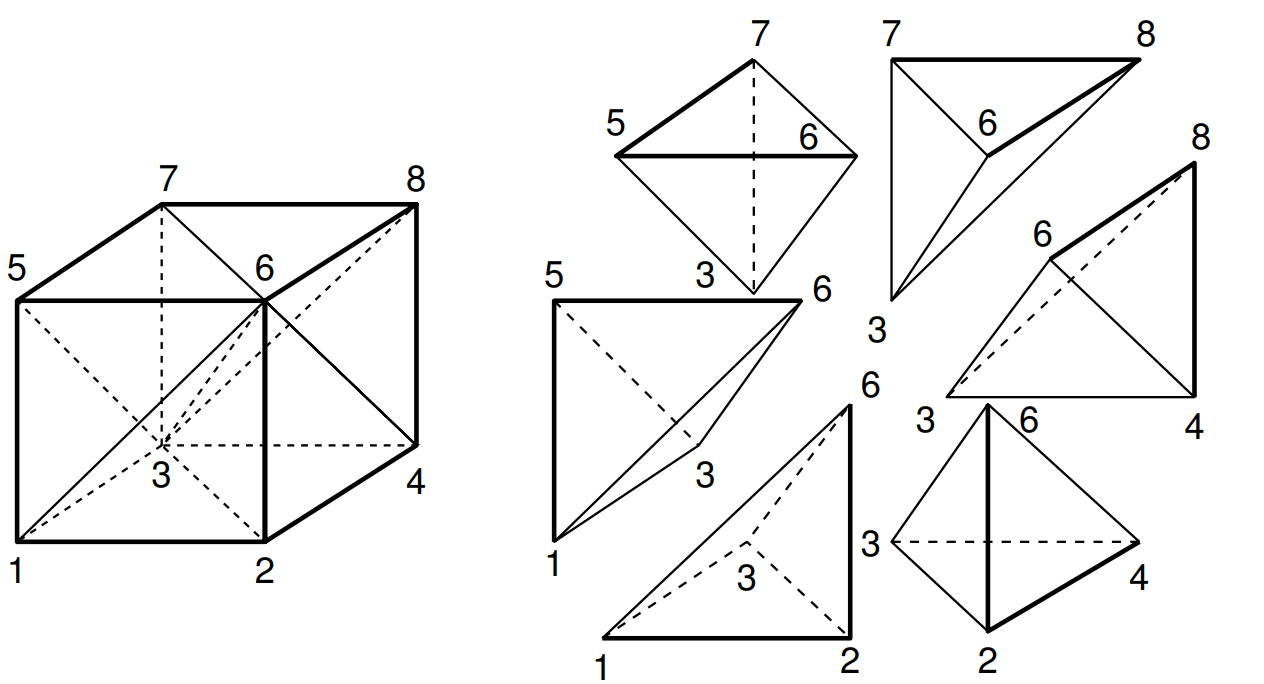
Then, the method assumes that, within a tetrahedron, the energy behaves linearly; therefore a linear interpolation is employed to obtain the value of the energy in any point inside the tetrahedron, knowing the values of the energy at its fours corners. Thanks to this, it is possible to calculate much more accurately the portion of the volume of each tetrahedron that is above or below a given energy, making the resulting DOS much more accurate than a simple histogram obtained from the value of the energy at its four corners.